A fairly recent blog post on the EGU blog site reiterated the compelling comparison between the current COVID-19 crisis and the ongoing climate emergency, focusing on extreme events such as hurricanes, heatwaves and severe rainfall-related flooding, all of which are likely to get worse as the climate warms (Langendijk & Osman 2020). This comparison has been made by us Climate Scientists since the COVID-19 crisis began; both the virus and the disastrous impacts of anthropogenic climate change were (and indeed are) predictable but little was done in the ways of preparedness, both were (and are still being) underestimated by those in power despite warnings from science, and both are global in extent and therefore require united action. Another comparison is that both are being intensively, and urgently, researched across the world by many centres of excellence. We don’t have all the answers yet for either, but progress is being made on both.
When it comes to understanding our climate, there are several approaches; these are, of course, not mutually exclusive. We can focus on present-day climate variability, to understand the physical mechanisms behind our current climate; examples include, but are not limited to, ocean-atmosphere interactions, land-atmosphere feedbacks, or extreme events (see Williams et al. 2008, Williams & Kniveton 2012 or Williams et al. 2012, as well as work from many others).
Alternatively, we can use our current understanding of the physical mechanisms driving current climate to make projections of the future, either globally or regionally. State-of-the-art General Circulation Models (GCMs) can provide projections of future climate under various scenarios of socio-economic development, including but not limited to greenhouse gas (GHG) emissions (Williams 2017).
A third approach is to focus on climates during the deep (i.e. geological) past, using tools to determine past climate such as ice cores, tree rings and carbon dating. Unlike the historical period, which usually includes the past in which there are human observations or documents, the deep past usually refers to the prehistoric era and includes timescales ranging from thousands of years ago (ka) to millions of years ago (Ma). Understanding past climate changes and mechanisms is highly important in improving our projections of possible future climate change (e.g. Haywood et al. 2016, Otto-Bliesner et al. 2017, Kageyama et al. 2018, and many others).
One reason for looking at the deep past is that it provides an opportunity to use our GCMs to simulate climate scenarios very different to today, and compare these to scenarios based on past.
These days I am primarily focusing on the latter approach, and am involved in almost all of the palaeoclimate scenarios coming out of UK’s physical climate model, called HadGEM3-GC3.1. These focus on different times in the past, such as the mid-Holocene (MH, ~6 ka), the Last Glacial Maximum (LGM, ~26.5 ka), the Last Interglacial (LIG, ~127 ka), the mid-Pliocene Warm Period (Pliocene, ~3.3 Ma) and the Early Eocene Climate Optimum / Paleocene-Eocene Thermal Maximum (EECO / PETM, collectively referred to here as the Eocene, ~50-55 Ma). All of these have been (or are being) conducted under the auspices of the 6th phase of the Coupled Modelling Intercomparison Project (CMIP6) and 4th phase of the Palaeoclimate Modelling Intercomparison Project (PMIP4).
These five periods are of particular interest to the above projects for a number of different reasons. Before these are discussed, however, the fundamentals of deep past climate change need to be briefly introduced. In short, climate changes in the geological past (i.e. without human influence) can either be internal to the planet (e.g. volcanic eruptions, oceanic CO2 release) or external to the planet (e.g. changes in the Earth’s orbit around the Sun). Arguably, it is changes to the amount of incoming solar radiation (known as insolation) that is the primary driver behind all long-term climate change. Theories for long-term climate change, such as the beginning and ending of ice ages, began to be proposed during the 1800s. However, it wasn’t until 1913 that the Serbian mathematician, Milutin Milankovitch, developed our modern day understanding of glacial cycles. In short, Milankovitch identified three interacting cycles concerning the Earth’s position relative to the Sun: a) Eccentricity, in which the Earth’s orbit around the Sun changes from being more or less circular on a period of 100-400 ka; b) Obliquity, in which the Earth’s axis changes from being more or less tilted towards the Sun on a period of ~41 ka; and c) Precession, in which the Earth’s polar regions appear to ‘wobble’ around the axis (like a spinning top coming to its end) on a period of ~19-24 ka. All of these three cycles not only change the overall amount of insolation received by the planet, and therefore its average temperature, but also where the most energy is received; this ultimately determines the strength and timing of our seasons.
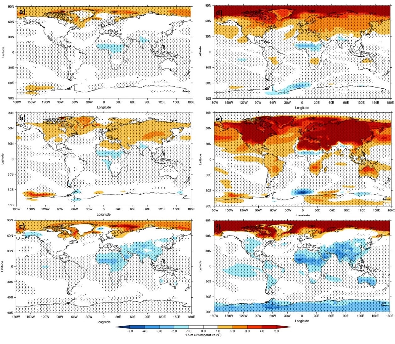
With this background in mind, and returning to the paleoclimate scenarios mentioned above, the MH and the LIG collectively represent a ‘warm climate’ state. During these periods the Earth’s axis was tilted slightly more towards the Sun, resulting in an increase in Northern Hemisphere insolation (because of the larger landmasses here relative to the Southern Hemisphere). This caused much warmer Northern Hemisphere summers and enhanced African, Asian and South American monsoons (Kageyama et al. 2018). The increase in temperatures can be seen in Figure 1, where clearly the largest increases relative to the preindustrial era (PI) are in the Northern Hemisphere during June-August (Williams et al. 2020). By comparing model simulations to palaeoclimate reconstructions during these periods, the models’ ability to simulate these climates can be tested and this therefore assesses our confidence in future projections of climate change; which, as mentioned above, may result in more rainfall extremes and enhanced monsoons.
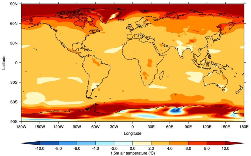
In contrast, the LGM represents a ‘cold climate’ state which, although unlikely to return as a result of increasing anthropogenic GHG emissions, nevertheless provides a well-documented climatic period during which to test the models. Going back further in time, the Pliocene is the most recent time in the geological past when CO2 levels were roughly equivalent to today, and was a time when global annual mean temperatures were 1.8-3.6°C higher than today (Haywood et al. 2016). See Figure 2 for the increases in sea surface temperature (SST) during the Pliocene, relative to today. This annual mean temperature increase is clearly much higher than the current target, as specified by the Paris Agreement, of keeping warming below 1.5°C (at most 2°C) by the end of 2100. Importantly, the CO2 increases and subsequent warming during the Pliocene occurred over timescales of thousands to millions of years, whereas anthropogenic GHG emissions have caused a similar increase in CO2 (from ~280 parts per million (ppmv) during the PI to just over 400 ppmv today) in under 300 years. The Pliocene, therefore, provides an excellent analogy for what our climate might be like in the (possibly near) future.
Finally, going back even further, the Eocene is the most recent time in the past that was characterised by very high CO2 concentrations, twice or more than that of today at >800-1000 ppmv; this resulted in temperatures ~5°C higher than today in the tropics and ~20°C higher than today at high latitudes (Lunt et al. 2012, Lunt et al. 2017). The reason the Eocene is highly relevant, and of concern, is that these CO2 concentrations are roughly equivalent to those projected to occur by the end of 2100, if the Representative Concentration Pathway (RCP) 8.5 scenario, also known as the ‘Business-as-usual’ scenario, which was used in the most recent IPCC report (IPCC 2014), becomes reality. The Eocene, therefore, provides an excellent albeit concerning analogy for what the worse-case scenario could be like in the future, if action is not taken.
 |
| Figure 2: 1.5 m air temperature climatology differences, Pliocene simulation from the UK’s physical climate model, relative to the preindustrial era. |
Understanding the climate, how it has changed in the past and how it might change in the future is a complex task and subject to various interrelated approaches. One of these approaches, the concept of using the past to inform the future (e.g. Braconnot et al. 2011), has been described here. Just like in the case of COVID-19, it is our responsibility as Climate Scientists to work together across approaches and disciplines, as well as reliably communicating the science to governments, policymakers and the general public, in order to mitigate the crisis as much as possible.
References
Braconnot, P., Harrison, S. P., Otto-Bliesner, B, et al. (2011). 'The palaeoclimate modelling intercomparison project contribution to CMIP5'. CLIVAR Exchanges Newsletter. 56: 15-19
Haywood, A. M., Dowsett, H. J., Dolan, A. M. et al. (2016). 'The Pliocene Model Intercomparison Project (PlioMIP) Phase 2: scientific objectives and experimental design'. Climate of the Past. 12: 663-675
IPCC (2014). 'Climate Change 2014: Synthesis Report. Contribution of Working Groups I, II and III to the Fifth Assessment Report of the Intergovernmental Panel on Climate Change' [Core Writing Team, R.K. Pachauri and L.A. Meyer (eds.)]. IPCC. Geneva, Switzerland, 151 pp
Kageyama, M., Braconnot, P., Harrison, S. P. et al. (2018). 'The PMIP4 contribution to CMIP6 – Part 1: Overview and over-arching analysis plan'. Geoscientific Model Development. 11: 1033-1057
Langendijk, G. S. & Osman, M. (2020). 'Hurricane COVID-19: What can COVID-19 tell us about tackling climate change?'. EGU Blogs: Climate. https://blogs.egu.eu/divisions/cl/2020/04/16/corona-2/. Accessed 24/7/20
Lunt, D. J., Dunkley-Jones, T., Heinemann, M. et al. (2012). 'A model–data comparison for a multi-model ensemble of early Eocene atmosphere–ocean simulations: EoMIP'. Climate of the Past. 8: 1717-1736
Lunt, D. J., Huber, M., Anagnostou, E. et al. (2017). 'The DeepMIP contribution to PMIP4: experimental design for model simulations of the EECO, PETM, and pre-PETM (version 1.0)'. Geoscientific Model Development. 10: 889-901
Otto-Bliesner, B. L., Braconnot, P., Harrison, S. P. et al. (2017). 'The PMIP4 contribution to CMIP6 – Part 2: Two interglacials, scientific objective and experimental design for Holocene and Last Interglacial simulations'. Geoscientific Model Development. 10: 3979-4003
Williams, C. J. R., Kniveton, D. R. & Layberry, R. (2008). 'Influence of South Atlantic sea surface temperatures on rainfall variability and extremes over southern Africa'. Journal of Climate. 21: 6498-6520
Williams, C. J. R., Allan, R. P. & Kniveton, D. R. (2012). 'Diagnosing atmosphere-land feedbacks in CMIP5 climate models'. Environmental Research Letters. 7 (4)
Williams, C. J. R. & Kniveton, D. R. (2012). 'Atmosphere-land surface interactions and their influence on extreme rainfall and potential abrupt climate change over southern Africa'. Climatic Change. 112 (3-4): 981-996
Williams, C. J. R. (2017). ‘Climate change in Chile: an analysis of state-of-the-art observations, satellite-derived estimates and climate model simulations’. Journal of Earth Science & Climatic Change. 8 (5): 1-11
Williams, C. J. R., Guarino, M-V., Capron, E. (2020). 'CMIP6/PMIP4 simulations of the mid-Holocene and Last Interglacial using HadGEM3: comparison to the pre-industrial era, previous model versions, and proxy data'. Climate of the Past. Accepted
--------------------------------
This blog was written by Cabot Institute member Dr Charles Williams, a climate scientist within the School of Geographical Sciences, University of Bristol. His research focusses on deep time to understand how climate has behaved in the warmer worlds experienced during the early Eocene and mid-Pliocene (ca. 50 – 3 Mio years ago). This blog was reposted with kind permission from Charles. View the original blog on the EGU blog site.
| Dr Charles Williams |

